%reload_ext autoreload
%autoreload 2
%matplotlib inline
Mixup
mixup can be thought of as a type of data augmentation. It was proposed in mixup: Beyond Empirical Risk Minimization to address some basic problems of empirical risk minimization (ERM - essentially, supervised machine learning).
One of the main problems they see is that:
ERM is unable to explain or provide generalization on testing distributions that differ only slightly from the training data.
Our data constricts what our model is able to learn. Even with complex neural networks the parameters can learn simple decision boundaries.
To overcome these issues they propose mixup:
In essence, mixup trains a neural network on convex combinations of pairs of examples and their labels. By doing so, mixup regularizes the neural network to favor simple linear behavior in-between training examples.#export
from exp.nb_12 import *
Data
path = datasets.untar_data(datasets.URLs.IMAGENETTE_160) # downloads and returns a path to folder
tfms = [make_rgb, ResizeFixed(128), to_byte_tensor, to_float_tensor] # transforms to be applied to images
bs = 128 # batch size
il = ImageList.from_files(path, tfms=tfms) # Imagelist from files
sd = SplitData.split_by_func(il, partial(grandparent_splitter, valid_name="val")) # Splitdata by grandparent folder function
ll = label_by_func(sd, parent_labeler, proc_y=CategoryProcesser()) # label the data by parent folder
data = ll.to_databunch(bs, c_in=3, c_out=10)
img1 = PIL.Image.open(ll.train.x.items[100])
img1

img2 = PIL.Image.open(il.items[2100])
img2

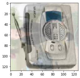
mixed_up = ll.train.x[100] * 0.3 + ll.train.x[2100] * 0.7
mixed_up
In a nutshell:
mixup constructs virtual training examples plt.imshow(mixed_up.permute(2,1,0))
Implementation
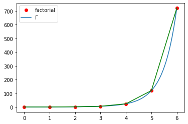
The gamma function can be seen as a solution to the following interpolation problem:
Find a smooth curve that connects the points $(x,y)$ given by $y=(x-1)!$ at the positive integer values for $x$
Basically, the gamma function using integral calculus to estimate how a smooth curve would connect the $(x,y)$ values of a factorial function.
Pytorch has a log gamma function which we can invert to make a gamma function.
$$ \text{out}_{i} = \log \Gamma(\text{input}_{i})$$Γ = lambda x: x.lgamma().exp()
facts = [math.factorial(i) for i in range(7)]
gamma = [torch.lgamma(i).exp() for i in torch.linspace(0,6, 7)+1]
plt.plot(range(7), facts, 'ro')
plt.plot(torch.linspace(0,6), Γ(torch.linspace(0,6)+1))
plt.plot(range(7), gamma, 'g')
plt.legend(['factorial','Γ']);
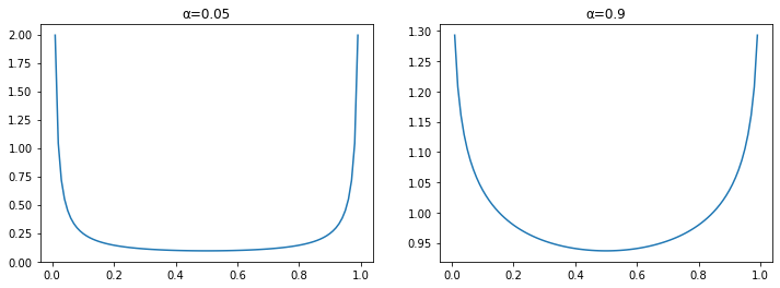
This is a smoothed histogram of how we are going to sample from the probability distribution:
_,axs = plt.subplots(1,2, figsize=(12,4))
x = torch.linspace(0,1, 100)
for α,ax in zip([0.05,0.9], axs):
    α = tensor(α)
    y = (x**(α-1) * (1-x)**(α-1)) / (Γ(α)**2 / Γ(2*α))
    ax.plot(x,y)
    ax.set_title(f"α={α:.1}")
nn.CrossEntropyLoss(
    weight=None,
    size_average=None,
    ignore_index=-100,
    reduce=None,
    reduction='mean',
)
Reduction:
(string, optional): Specifies the reduction to apply to the output: ``'none'`` | ``'mean'`` | ``'sum'``. ``'none'``: no reduction will be applied, ``'mean'``: the sum of the output will be divided by the number of elements in the output, ``'sum'``: the output will be summed. Note: :attr:`size_average`#export
class NoneReduce():
def __init__(self, loss_func):
self.loss_func = loss_func
self.old_red = None
def __enter__(self):
if hasattr(self.loss_func, 'reduction'):
self.old_red = getattr(self.loss_func, "reduction")
setattr(self.loss_func, "reduction", "none")
return self.loss_func
else: return partial(self.loss_func, reduction='none')
def __exit__(self, type, value, traceback):
if self.old_red is not None:
setattr(self.loss_func, 'reduction', self.old_red)
Mixup
#export

from torch.distributions.beta import Beta

def unsqueeze(input, dims):
    for dim in listify(dims): input = torch.unsqueeze(input, dim)
    return input

def reduce_loss(loss, reduction='mean'):
    return loss.mean() if reduction=='mean' else loss.sum() if reduction=='sum' else loss

def lin_comb(v1, v2, beta): return beta*v1 + (1-beta)*v2
#export
class MixUp(Callback):
    _order = 90 #Runs after normalization and cuda
    def __init__(self, α:float=0.4): self.distrib = Beta(tensor([α]), tensor([α]))

    def begin_fit(self): self.old_loss_func,self.run.loss_func = self.run.loss_func,self.loss_func

    def begin_batch(self):
        if not self.in_train: return #Only mixup things during training
        λ = self.distrib.sample((self.yb.size(0),)).squeeze().to(self.xb.device)
        λ = torch.stack([λ, 1-λ], 1)
        self.λ = unsqueeze(λ.max(1)[0], (1,2,3))
        shuffle = torch.randperm(self.yb.size(0)).to(self.xb.device)
        xb1,self.yb1 = self.xb[shuffle],self.yb[shuffle]
        self.run.xb = lin_comb(self.xb, xb1, self.λ)

    def after_fit(self): self.run.loss_func = self.old_loss_func

    def loss_func(self, pred, yb):
        if not self.in_train: return self.old_loss_func(pred, yb)
        with NoneReduce(self.old_loss_func) as loss_func:
            loss1 = loss_func(pred, yb)
            loss2 = loss_func(pred, self.yb1)
        loss = lin_comb(loss1, loss2, self.λ)
        return reduce_loss(loss, getattr(self.old_loss_func, 'reduction', 'mean'))
nfs = [32,64,128,256,512]
def get_learner(nfs, data, lr, layer, loss_func=F.cross_entropy,
                cb_funcs=None, opt_func=optim.SGD, **kwargs):
    model = get_cnn_model(data, nfs, layer, **kwargs)
    init_cnn(model)
    return Learner(model, data, loss_func, lr=lr, cb_funcs=cb_funcs, opt_func=opt_func)
cbfs = [partial(AvgStatsCallback,accuracy),
        CudaCallback,
        ProgressCallback,
        partial(BatchTransformXCallback, norm_imagenette),
        MixUp]
learn = get_learner(nfs, data, 0.4, conv_layer, cb_funcs=cbfs)
learn.fit(20)
Let's change the mixup alpha parameter:
cbfs = [partial(AvgStatsCallback,accuracy),
        CudaCallback,
        ProgressCallback,
        partial(BatchTransformXCallback, norm_imagenette),
        partial(MixUp, α=0.8)]
learn = get_learner(nfs, data, 0.3, conv_layer, cb_funcs=cbfs)
learn.fit(20)
nb_auto_export()